From Near-Field Measurements to Far-Field Predictions: A Machine Learning Approach in EOL Testing
By Dani Fernández Comesaña, Matheus Lazarin, Enzo Brusque Bom of Microflown Technologies, Netherlands and Cástor Rodríguez, Sound of Numbers, Spain
Ensuring product quality through effective End-Of-Line (EOL) testing is a critical aspect of modern manufacturing. Traditional acoustic testing methods often face challenges in noisy factory environments, particularly when attempting to replicate free-field conditions for far-field sound pressure measurements. This article explores a novel approach that integrates near-field particle velocity measurements with machine learning (ML) algorithms to predict far-field acoustic behavior and detect manufacturing defects. Leveraging the Kirchhoff–Helmholtz integral theorem, this method reconstructs sound pressure at any point using near-field data combined with acoustic transfer functions. The integration of ML algorithms facilitates the classification of various quality defects based on the rich information inherent in particle velocity data, offering a scalable solution effective even with small sample sizes. This methodology not only streamlines the EOL testing process but also ensures that acoustic performance standards are consistently met for every single manufactured product.
Advancements with Particle Velocity Sensors
Unlike traditional sound pressure, particle velocity is a vector quantity, offering both magnitude and directional information of the sound field. In practice, the direct measurement of this quantity using a dedicated sensor [1,2] yields several advantages [3,4], such as:
- Proximity Measurements: Positioning particle velocity sensors close to the noise-emitting surfaces of a device enhances the signal-to-noise ratio due to near-field effects, facilitating accurate measurements even in environments with high background noise.
- Surface Displacement Correlation: Particle velocity data measured near the device surface is proportional to surface displacement, providing key information about the structural behavior of the device under test.

Figure 1- MEMS particle velocity sensor
Calculating Far-Field Sound Pressure from Near-Field Particle Velocity
Understanding the noise emitted by a device at a certain distance is often a requirement for most EOL acoustic testing stations. The sound pressure Pref located at the reference position 𝐱 due to a continuous rigid radiating surface S can be derived from the simplified Kirchhoff-Helmholtz Integral Equation [5], i.e.

where un(𝐲) is the normal particle velocity at position 𝐲 on the surface S and G(𝐱,𝐲) is the Green function that relates the propagation between the points 𝐱 and 𝐲. In practical scenarios, it is often necessary to reconstruct the far-field sound pressure using a (very) limited number of near-field measurements. To achieve reconstructions with a minimal number of sampling points, one effective approach involves matrix inversion using experimental data, obtaining a set of weighting functions h(𝐱,𝐲𝐍), i.e.

Figure 2- Schematic representation of the sound pressure prediction system (left) and experimental results (right)
Once the far-field sound pressure has been predicted, traditional acoustic quality criteria can be applied. Compliance with defined acoustic performance standards—such as tolerance limits on spectral content or time signals—can then be easily verified using the reconstructed far-field data. This approach effectively integrates traditional EOL evaluation criteria into a flexible testing procedure implemented directly on the production line.
Enhancing EOL Testing with Machine Learning
Nowadays, several AI/ML algorithms are available for enhancing the accuracy and reliability of end-of-line (EOL) testing. Among these techniques, the usage of a Gaussian Mixture Model (GMM) stands out due to its flexibility and effectiveness. This methodology has proven highly effective in practical applications [6,7], especially when deploying EOL systems for new products, where comprehensive acoustic datasets are typically scarce. Early-stage products often undergo significant design changes, making it challenging to collect extensive recordings with a consistent acoustic output. By defining fault-specific features from near-field particle velocity measurements, a preliminary yet robust statistical model can be established at early product stages, requiring only a minimal number of sample units.

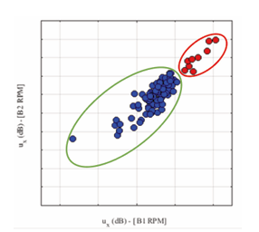
Figure 3 – 2D feature analysis results with sound pressure (top) and particle velocity (bottom) features.
Figure 3 illustrates a practical application of this approach. Features extracted from measurements taken at two operational load conditions (rotational speeds B1 on the x-axis and B2 on the y-axis) are compared. Gaussian Mixture Model boundaries clearly distinguish two classes: “Good Samples,” shown in green, and “Defective Samples,” highlighted in red. By analyzing data from sound pressure microphones and particle velocity sensors, the differences in classification performance become evident. While sound pressure data shows some ambiguity and potential misclassification, the data derived from particle velocity sensors provides clear and unambiguous differentiation between good and defective samples.
The superior performance observed with particle velocity data is due to its direct relationship with surface displacement, resulting in greater source identifiability and improved separation of acoustic contributions from individual device components. This enhances the capability of machine learning algorithms, such as GMM, to reliably classify defects.
Conclusion
The integration of particle velocity sensors and machine learning algorithms has significantly advanced the field of acoustic EOL testing. This combination allows for accurate, efficient, and comprehensive testing directly within manufacturing environments, even in the presence of high background noise. Manufacturers can now ensure that their products meet stringent acoustic performance standards, enhancing customer satisfaction and reducing the likelihood of costly recalls or reputational damage. For more information see the references, and also our webinar on ‘How to Design A Successful End-of-line Quality Control System’.
References
- de Bree, H. E., “The Microflown”. PhD Thesis, University of Twente, the Netherlands, 1997.
- Acoustic Particle Velocity Sensors, online: https://www.microflown.com/products/acoustic-particle-velocity-sensors
- Fernandez Comesana, D., Yang, F., Tijs, E., “Influence of background noise on non-contact vibration measurements using particle velocity sensors”, INTER-NOISE and NOISE-CON Congress and Conference Proceedings, pp. 1871-1876(6), 2014.
- Fernandez Comesana, D., Cereijo Graña, I., Grosso A., “Particle velocity sensors for enhancing vehicle acoustic simulations” in Proceedings of AIA-DAGA, pp. 1236-1239, 2013.
- E. G. Williams, “Fourier Acoustics: Sound Radiation and Nearfield Acoustical Holography,” Academic Press, 1999.
- Carrillo Pousa, G., Fernandez Comesana, D. and Wild, J., “Acoustic particle velocity for fault detection of rotating machinery using tachless order analysis,” in Inter-Noise, 2015.
- Fernandez Comesana, D., Carrillo Pousa, G., and Tijs, E., ” Integration of an End-of-Line System for Vibro-Acoustic Characterization and Fault Detection of Automotive Components Based on Particle Velocity Measurements,” SAE Technical Paper 2017-01-1761, 2017, doi:10.4271/2017-01-1761.